
Well, our aim is understand the factors that determine speed of a bicycle and to estimate the speed for a realistic case. We will begin with ignoring air friction.
From Newton's second law, the equation of motion can be written in the form:
|
(1) |
where  is the velocity,
 is the mass of the bicycle-rider
combination,
is the mass of the bicycle-rider
combination,  is the time, and
 is the force on the bicycle
that comes from the effort on the rider. Using work-energy theorem
the power output,
is the force on the bicycle
that comes from the effort on the rider. Using work-energy theorem
the power output,  , of the rider can be
calculated from:
, of the rider can be
calculated from:
 |
(2) |
Inserting Equation (2) into (1) yields:
 |
(3) |
Analitic solution of this differential equation (assuming
is constant) is:
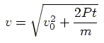 |
(4) |
where  is the velocity of the
bicycle at = 0.
Equation (4) is unphyiscal since it predicts that the velocity will
increasewitout bound at long times.
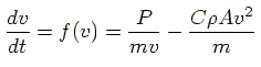
If we consider the effect of the air resistance force that is atmosferic drag,
model becomes realistic. In general this force can be written
form:
is the velocity of the
bicycle at = 0.
Equation (4) is unphyiscal since it predicts that the velocity will
increasewitout bound at long times.
If we consider the effect of the air resistance force that is atmosferic drag,
model becomes realistic. In general this force can be written
form:
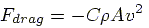 |
(5) |
where  is known as the drag coefficient,
 is the air density and
 is the frontal area of
the rider. If we add the drag force into differantial equation (3) then:
is the frontal area of
the rider. If we add the drag force into differantial equation (3) then:
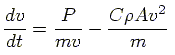 |
(6) |
Numerical solution of this diffrential equation can be develop by using secon order Runge-Kutta Method. In general Equation (6) has the form:
 |
(7) |
General Runge-Kutta solution steps for this kind of equation are:
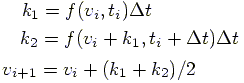 |
(8) |
where  is the small discrete time steps.
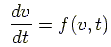
In fact, the right hand side of the Equation (6) does not contain
time, . Differential equation
and reduce to:
is the small discrete time steps.
In fact, the right hand side of the Equation (6) does not contain
time, . Differential equation
and reduce to:
 |
(9) |
and corresponding Runge-Kutta steps:
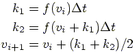 |
(10) |
The typical physical parameters and the computer programs in Fortran 90
and ANSI C can be found at:
bicycleRacer.f90 |
bicycleRacer.c
The results obtained from numerical solution of Equation (9) is shown
in Figure given below for diffrent values
.
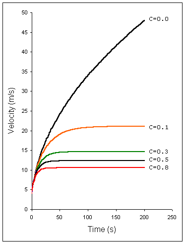
Velocity as a function of time for the different values of drag coefficient,
C.