A Toy Monte Carlo Simulation of ECAL Dectector
Physics of an ECAL Dectector
The energy and position coordinates of secondaries from high-energy interactions
can also, under suitable conditions, be measured by total absorption
methods. In the absorption process, the incident particle interacts in a large
detector mass, generating secondary particles which in turn generate tertiary
particles, and so on, so that all (or most) of the incident energy appears as
ionisation or excitation in the medium-hence the term calorimeter [Perkins].
|
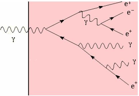
For electrons and photons of high energy, a dramatic result of the combined
phenomena of bremsstrahlung and pair production is the occurance of cascade
showers. A parent will radiate photons, which convert to pair, which radiate and
produce fresh pairs in turn, the number of particle increasing exponentially with
depth in the medium. A measurement of the position and charge of a shower
provides a measure of the position an energy of the electron or photon [Perkins].
An example of a photon enetering an ECAL and producing a shower is shown in the figure
given right.
|
|
In High Energy Experiments, ECAL is used to measure energy of an electron or photon.
ECAL energy calibration procedure uses electrons or photons from different sources.
The energy resolution of an ECAL, can be determined by comparing the measured energy to
the track momentum. An example is shown in figure below (as a function of track energy)
for the ALEPH ECAL detector used at LEP.
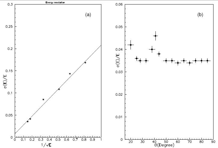 The corresponding fitted resolution is:
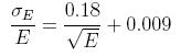 where E is measured inGeV. General form of the form of this equation is:
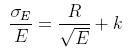 where R is called stochastic term (slope) and k is the constant term (intercept).
For ALEPH detector at LEP: R=0.18 and k=0.009
For ATLAS detector at LHC: R=0.10 and k=0.007
For CMS detector at LHC: R=0.04 and k=0.005
Another important parameter of an ECAL is spatial (angular) resolution. General form is:
 where A and B are constrant and has the typical values A = 10 mrad.GeV1/2 and B = 0.1 mrad.
Simulation
We can perform a toy simulation for an ECAL as follows:
- Energy resolution is simulated by Gaussian smearing the energy of photons; the relative
energy resolution has the form for example: sigma(E) = 10%/sqrt(E)
- Spatial resolution is simulated by Gaussian smearing the angular position of photons; the
angular resolution has the form for example sigma(theta,phi) = 40 mrad/sqrt(E).
Example Application
Here we will show the importance of the resolution effects of an ECAL on the photons.
Consider the decay: pi0 -> gamma1 + gamma2. We can generate, using Monte Carlo, these photons
and pass them to an ECAL to reconstruct their energies. That is basicly to say,
four-momenta of the generated and reconstructed photons will be different. We can see the effect of
ECAL on the invariant mass of photons, m(gamma1,gamma2). Figure shows
two plots of two-photon invariant mass (m) of two photons originating from a pi0 with and without ECAL simulation.
After applying the smearings, the pi0 invariant mass has distribution instead of a simple spike.
The computer implementations:
ecalBasic.cpp |
ecalBasic.cxx (ROOT)
See also:
Random.h |
Particle.h |
Detector.h