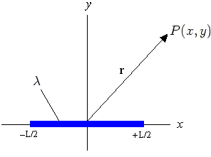
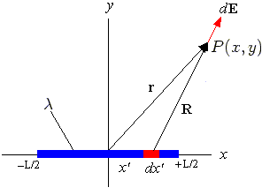
Electric Field Near a Straight Line Charge
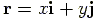
and  is the unit vector in the
direction of the vector
is the unit vector in the
direction of the vector  . Putting
 , Equation (1) becomes:
 |
(3) |
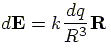
By using vector a operation, the vector
can be written in terms of position vector
 such that:
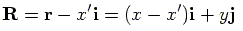 |
(4) |
and the length of can be expressed as a
function of geometric parameters:
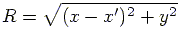 |
(5) |
The charge of the segment,  ,
can be written as:
,
can be written as:
 |
(6) |
Subsitution of Equations (4), (5) and (6) into Equation (3) yields:
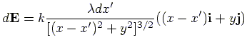 |
(7) |
The total electric field,  , is the
integral of electric field
, is the
integral of electric field  over the wire.
So, the componets of
are found by evaluating the following integrals:
over the wire.
So, the componets of
are found by evaluating the following integrals:
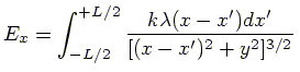 |
(8) |
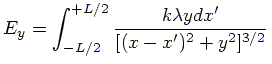 |
(9) |
In our program, we will evaluate these integrals numerially.
Integrating a function  can be calculated by
Simpson's method.
The approximation to the integral is:
can be calculated by
Simpson's method.
The approximation to the integral is:
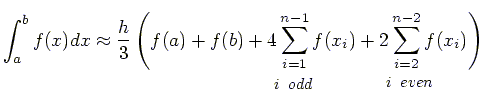 |
(10) |
where  is a finite length of
 . Note that numerical errors can be
reduced by making smaller.
The Simpson method in Equation (10) is used to solve the integrals
in Equation (8) and (9).
. Note that numerical errors can be
reduced by making smaller.
The Simpson method in Equation (10) is used to solve the integrals
in Equation (8) and (9).
The computer programs in Fortran 90 and C can be found at:
linearCharge.f90 |
linearCharge.c
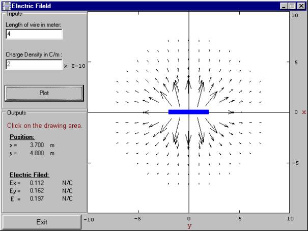
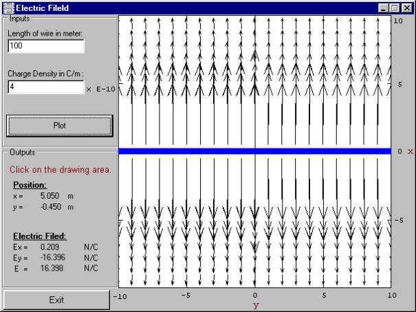
You can also download an executable visual program file produced by
Borland C++ Builder 1.0 from: linearCharge.exe
You can input  and
and
 parameters and the program
plots the 2D-distribution of the electric field vectors,
.
parameters and the program
plots the 2D-distribution of the electric field vectors,
.
Secreen Shots:
02_1.jpg |
02_2.jpg |
02_3.jpg
 produced by a charged wire whose length is
 from it, is calculated from:
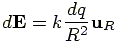
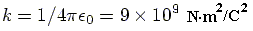
 is a constant
and has the value:
is a constant
and has the value: